H3-Boundary¶

Boundary cells and boundary polygons for Uber's H3 grid.

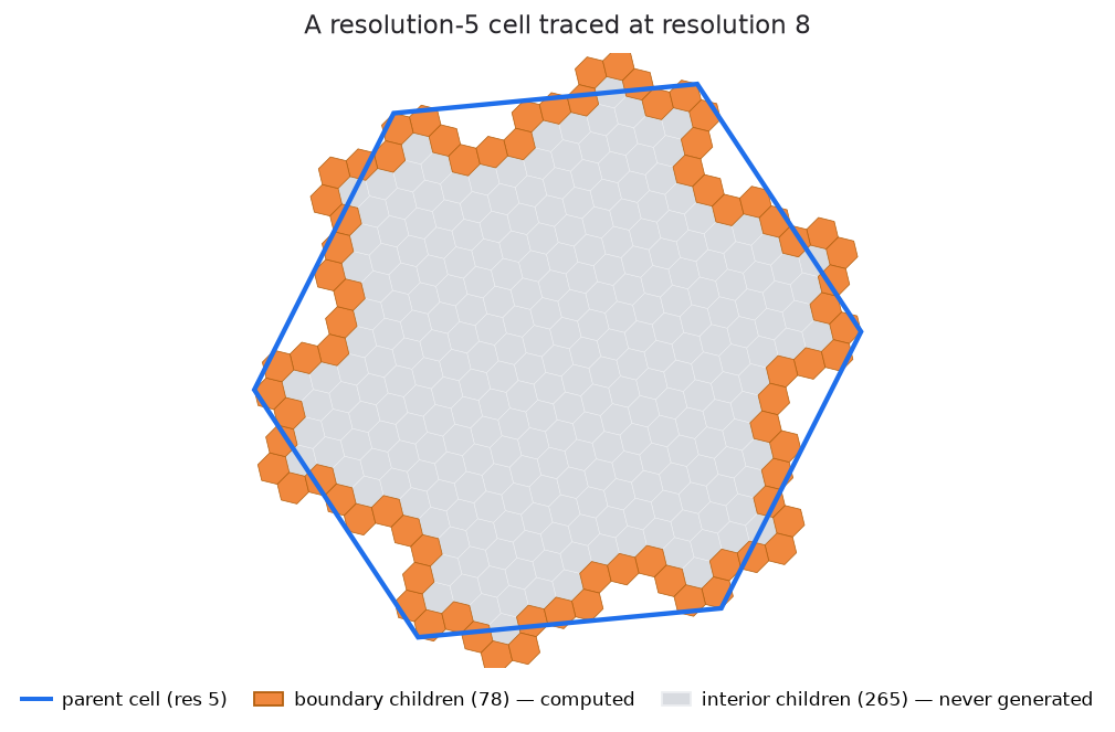
An H3 cell at one resolution contains thousands — or billions — of cells at finer resolutions. H3-Boundary works with the ones on its edge: it lists them, traces their outline, and builds polygons that safely contain them. Cost scales with the boundary, never with the interior.

A resolution-5 H3 cell traced at resolution 8: its 78 boundary cells highlighted, its 265 interior cells greyed out

pip install h3-boundary

Quick start¶

Start from any H3 cell. Here we index downtown San Francisco at resolution 6 — a district-sized cell of about 36 km² — using latlng_to_cell from h3-py, which H3-Boundary already depends on.

import h3
import h3_boundary as h3b

cell = h3.latlng_to_cell(lat=37.7759, lng=-122.4180, res=6)

# 1. Its boundary cells: the descendants at resolution 10 (block-sized cells)
#    that lie on its edge
edge = h3b.children_on_boundary_faces(cell, target_res=10)
len(edge)                                                # 240, out of 2,401 descendants

# 2. Its exact outline — the shape those descendants actually fill
outline = h3b.cell_boundary_from_children(cell, target_res=10)

# 3. That same outline, grown by a safety margin
safe = h3b.get_buffered_boundary_polygon(cell, intermediate_res=10)
safe["properties"]["buffer_meters"]                      # 75.9 — the margin added

Both polygons are GeoJSON Features, and both trace the boundary at resolution 10 — the difference is what they are for. The outline is the exact shape: draw it. On its own it is not safe to filter with, because cells finer than resolution 10 still poke slightly past it; safe pushes the edges out by one resolution-10 edge length (75.9 m), after which nothing can fall outside at any resolution. That is also why its parameter is called intermediate_res — there, tracing is only an intermediate step.

Why not just use the hexagon H3 draws for the cell? Because that hexagon is not where the descendants sit — they straddle it, as the figure above shows. Filtering fine-resolution data with it silently loses the cells along the edge (about 7% of them). Buffered Polygons has the full story.

Working at scale¶

Interiors explode; boundaries stay manageable. Boundary size has a closed form — 3**(depth + 1) - 3, where depth is how many resolution levels you descend — so it is known before computing anything. A resolution-2 cell has close to two billion descendants at resolution 13, but only 531,438 of them lie on its boundary, and you never need to build even those to use them:

res, target = 2, 13                          # a country-sized cell, traced with ~44 m² cells
big = h3.latlng_to_cell(lat=37.7759, lng=-122.4180, res=res)

depth = target - res                         # 11 levels of subdivision between the two
total = 3 ** (depth + 1) - 3                 # 531,438 boundary cells, known without counting

ids = h3b.boundary_cell_ids(big, target_res=target)               # all of them, uint64, ~4 ms
mid = h3b.boundary_cell_at(big, target_res=target, n=total // 2)  # any one, in microseconds
h3b.boundary_rank(big, mid)                                       # the inverse — also a membership test
h3b.boundary_range(big, target_res=target, start=0, stop=100)     # any slice — stream it, or shard it

Disjoint slices reassemble into exactly the full boundary, so parallel workers need no coordination. Boundary Indexing explains how single cells are computed directly.

Performance¶

Measured on Linux / Python 3.14; the C++ extension is used automatically when present.

Operation	Boundary size	Time
Boundary cells — `children_on_boundary_faces`	240	0.02 ms
Boundary cells, large — `boundary_cell_ids`	531,438	4 ms
One cell by index — `boundary_cell_at`	any	0.014 ms
Boundary polygon — `cell_boundary_from_children`	240	1.6 ms
Buffered polygon, accurate	240	6 ms
Buffered polygon, convex hull	240	0.4 ms

boundary_cell_at costs the same whether the boundary holds 78 cells or half a million.

Guides¶

Page	What's in it
Interactive Demo	Boundary tracing and buffering, on a map
Concepts	How boundary tracing works
Boundary Algorithms	Four ways to compute boundary cells, compared
Boundary Indexing	How the n-th boundary cell is computed directly
Buffered Polygons	Why buffering is needed, and what each mode guarantees
API Reference	Every function

Notebooks¶

Three runnable demos live in notebook/ — clone the repo and open them with jupyter notebook:

Notebook	What it shows
`demo_generation.ipynb`	Boundary tracing and buffering step by step, each stage drawn on a map
`boundary_indexing_demo.ipynb`	Large boundaries: bulk ids, reaching one cell directly, sharding
`buffered_polygon_demo.ipynb`	The three buffering modes compared, with a containment check for each

Installation¶

Ships as a source distribution. During install it compiles a C++ extension if cmake, a C++17 compiler and the Boost headers are present; otherwise it installs pure-Python and every function still works, just more slowly. Same results either way, verified by a parity test suite.

import h3_boundary

h3_boundary.get_backend()        # 'cpp' or 'python'
h3_boundary.cpp_geom_available() # True if the C++ geometry functions exist

License¶

MIT — see LICENSE.